Skip to content
2D Multi-Body Physics Engine
Python | Machine Dynamics | Lagrangian Mechanics | Impact Simulation
Project Overview
Northwestern University’s Mech_Eng 314 – Machine Dynamics class covers the the foundations of rigid multi-body Lagrangian Mechanics. Students taking this class model complex dynamic rigid body interactions such as impacts, constraints, and external forces using numerical methods.
For the final project, students model, simulate, and animate a dynamic multi body system using Python’s numpy, sympy, and plotly packages. I chose to model a Dice in Cup (Jack in the box) system. The cup is subject to oscillating external forces to mimic a person shaking it, while the die is constrained to bounce around inside the cup.
Simulation Video
System Modelling
The system comprises two rigid bodies, the die and the cup, each with 3 degrees of freedom (in-plane translation and rotation) in the 2D plane.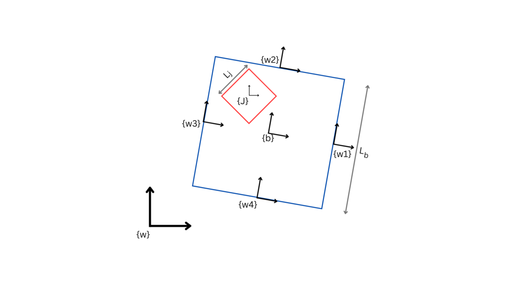
List of Rigid Body Transformations:
$$
g_{wj} =\begin{bmatrix}\cos \theta_j(t) & -\sin \theta_j(t) & 0 & x_j(t) \\ \sin \theta_j(t) &
\cos \theta_j(t)& 0 & y_j(t)\\ 0 & 0 & 1 & 0\\ 0 & 0 & 0 & 1\end{bmatrix},\:\:\:\:
g_{wb} =\begin{bmatrix}\cos \theta_b(t) & -\sin \theta_b(t) & 0 & x_b(t) \\ \sin \theta_b(t) &
\cos \theta_b(t)& 0 & y_b(t)\\ 0 & 0 & 1 & 0\\ 0 & 0 & 0 & 1\end{bmatrix}\\
$$
$$
g_{bw1} =\begin{bmatrix}1 & 0 & 0 & L_b/2 \\ 0 &
1& 0 & 0\\ 0 & 0 & 1 & 0\\ 0 & 0 & 0 & 1\end{bmatrix},\:\:\:\:
g_{bw2} =\begin{bmatrix}1 & 0 & 0 & 0 \\ 0 &
1& 0 & L_b/2\\ 0 & 0 & 1 & 0\\ 0 & 0 & 0 & 1\end{bmatrix},\:\:\:\:
g_{bw3} =\begin{bmatrix}1 & 0 & 0 & -L_b/2 \\ 0 &
1& 0 & 0\\ 0 & 0 & 1 & 0\\ 0 & 0 & 0 & 1\end{bmatrix},\:\:\:\:
g_{bw4} =\begin{bmatrix}1 & 0 & 0 & 0 \\ 0 &
1& 0 & -L_b/2\\ 0 & 0 & 1 & 0\\ 0 & 0 & 0 & 1\end{bmatrix}
$$
The transforms between the world and the walls are calculated using:
$$
g_{ww1} = g_{wb}g_{bw1}, \:\:\:\:g_{ww1} = g_{wb}g_{bw1},\:\:\:\:g_{ww1} = g_{wb}g_{bw1},\:\:\:\:g_{ww1} = g_{wb}g_{bw1}
$$
Problem Solving procedure:
1. Define the transforms as per the system model diagram.
2. Calculate the kinetic and potential energies of the system.
3. Compute the Lagrangian using:
$$
L = KE_{b}+KE_{j} – (V_{b}+V_{j})
$$
4. The euler lagrange equations are calculated using:
$$
\frac{d}{dt}\left(\frac{\partial L}{\partial \dot{q}}\right) – \frac{\partial L}{\partial q} = F
$$
5. Where external forcing on the box is defined as:
$$
F_x = -k_x \cdot (x_b – A_x \sin(2\pi t)) \\
F_y = m_b \cdot g – k_y\cdot y_b \\
F_\theta = -k_\theta \cdot \theta_b
$$
Fx is an oscillating force in the x direction, Fy offsets gravity and applies a restoring force for displacements in the y direction like a linear spring and Ftheta applies a restoring force for angular displacements like a torsion spring.
6. Solve the Euler-Lagrange equations and lambdify the solutions.
7. For calculating constraints, define the four corners of the jack in the jack frame. Compute their positions in the wall frames to get the constraint expressions. Jack corners are defined as:
$$
\begin{bmatrix}
\frac{L_j}{\sqrt{2.0}} \\
0 \\
0 \\
1
\end{bmatrix}, \quad
\begin{bmatrix}
0 \\
\frac{L_j}{\sqrt{2.0}} \\
0 \\
1
\end{bmatrix}, \quad
\begin{bmatrix}
-\frac{L_j}{\sqrt{2.0}} \\
0 \\
0 \\
1
\end{bmatrix}, \quad
\begin{bmatrix}
0 \\
-\frac{L_j}{\sqrt{2.0}} \\
0 \\
1
\end{bmatrix}
$$
If wall ID is 0 or 2, the jack corner in the corresponding wall frame is obtained by:
$$
\begin{bmatrix}
1 & 0 & 0 & 0
\end{bmatrix}
\cdot g_{w1w} \cdot g_{wj} \cdot
\begin{bmatrix}
\frac{L_j}{\sqrt{2.0}} \\
0 \\
0 \\
1
\end{bmatrix}
$$
If wall ID is 1 or 3, the jack corner in the corresponding wall frame is obtained by:
$$
\begin{bmatrix}
0 & 1 & 0 & 0
\end{bmatrix}
\cdot g_{w2w} \cdot g_{wj} \cdot
\begin{bmatrix}
\frac{L_j}{\sqrt{2.0}} \\
0 \\
0 \\
1
\end{bmatrix}
$$
8. These lambdified contraint expressions are stored in a list and are numerically evaluated at each timestep to detect impact.
9. The impact detection function monitors for a change in sign when evaluating the impact conditions for the current and next timestep. If an impact is detected, the impact update function is called.
10. The impact update laws are calculated using the equations given below:
$$
\begin{aligned}
\frac{\partial L}{\partial \dot{q}} \Big\vert^{\tau^+}_{\tau^-} & = \lambda \frac{\partial \phi}{\partial q} \\
\left[ \frac{\partial L}{\partial \dot{q}}\cdot\dot{q} – L(q,\dot{q}) \right] \Bigg\vert^{\tau^+}_{\tau^-} & = 0
\end{aligned}
$$
11. The impact update equations for wall/corner pair are stored in a list. When an impact is detected, the impact update function fetches the corresponding update equations from this list and computes the post impact velocites.
Note on handling Simultaneous Impacts:
Upon detecting simultaneous impacts, the system’s updated state, derived from solving the first set of impact update equations, is used as input for the next set of impact equations and so on. This method addresses a specific subset of simultaneous impacts, though it does not cover all scenarios.
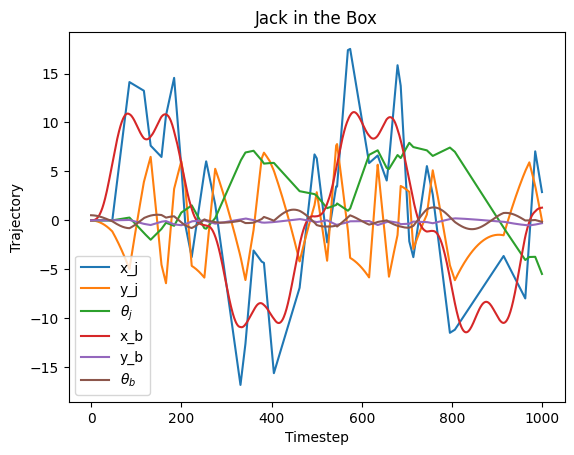
Description of Simulation:
When the simulation begins, the jack falls under the effect of gravity, while the box moves under the influence of the external forcing (F). The plot clearly shows that the box oscillates in the X direction, doesn’t move much in the Y direction due to the linear spring and tries to return to its natural angular orientation beacuse of the restoring force from the torsion spring. The jack experiences multiple impacts, and the motions of both the jack and the box are consistent with our physical intuition about this system.