KUKA youBot Mobile Manipulator

Python | Kinematics | Screw Theory | Feedback Control | Trajectory Generation | Path Planning | CoppeliaSim

Project Overview

For this project, I wrote software that plans a trajectory for the end-effector of the KUKA youBot mobile manipulator (a mobile base with four mecanum wheels and a 5R robot arm), performs odometry as the chassis moves, and implements Feedforward + PI control to drive the youBot to pick up a block at a specified location, carry it to a desired location, and put it down. This project uses the CoppeliaSim physics simulator to simulate the interaction between the youBot and objects in the environment (in this case a simple cube). The full project description can be found here.

KUKA youBot Mobile Manipulator executing a Pick-and-Place action

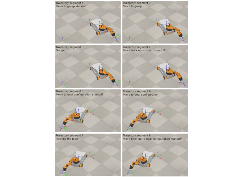
The program takes as input:

  • the initial resting configuration of the cube object (which has a known geometry), represented by a frame attached to the center of the object
  • the desired final resting configuration of the cube object
  • the actual initial configuration of the youBot (given by a 13-vector)
  • the initial configuration  of the reference trajectory for the end-effector frame of the youBot

The  output of the program is:

  • a csv file which, when “played” through the CoppeliaSim scene, drives the youBot to successfully pick up the block and put it down at the desired location
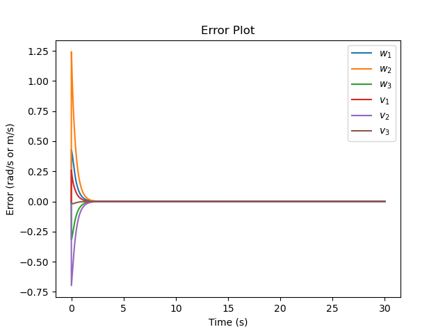
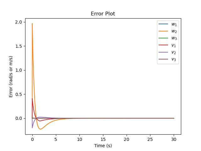
  • a data file containing the 6-vector end-effector error (the twist that would take the end-effector to the reference end-effector configuration in unit time) as a function of time

The configuration of the robot at time \(t\) is represented as a thirteen vector: $$q = \begin{bmatrix} \phi_{chassis} \\
x_{chassis} \\
y_{chassis} \\
J_1 \\
J_2 \\
J_3 \\
J_4 \\
J_5 \\
W_1 \\
W_2 \\
W_3 \\
W_4 \\
\text{gripper state} \end{bmatrix}$$

where \( \phi_{chassis},
x_{chassis},
y_{chassis}\) represent the chassis pose, \(J_1\) to \(J_5\) are the arm joint angles, \(W_1\) to \(W_4\) are the four wheel angles and gripper state {0 or 1} indicates whether the gripper is open or closed.

Using the program inputs, a reference trajectory for the pick-and-place task is generated in 8 distinct segments:

  1. A trajectory to move the gripper from its initial configuration to a “standoff” configuration a few cm above the block.
  2. A trajectory to move the gripper down to the grasp position.
  3. Closing of the gripper.
  4. A trajectory to move the gripper back up to the “standoff” configuration.
  5. A trajectory to move the gripper to a “standoff” configuration above the final configuration.
  6. A trajectory to move the gripper to the final configuration of the object.
  7. Opening of the gripper.
  8. A trajectory to move the gripper back to the “standoff” configuration.
KUKA youBot reference trajectory generation for pick-and-place application

The NextState() function in the codebase takes as input:

  • a 13-vector representing the current configuration of the robot
  • a 9-vector of controls indicating the wheel speeds \(u\)(4 variables) and the arm joint speeds \(\dot{\theta}\) (5 variables)
  • a timestep \(\Delta t\)

and outputs a 13-vector representing the configuration of the robot time \(\Delta t\)  later.


The FeedbackControl() function calculates the kinematic task-space feedforward plus feedback control signal which is defined as:


$$\mathcal{V}(t) = [Ad_{X^{-1}X_{d}}]\mathcal{V}_{d}(t) + K_{p}X_{err}(t) + K_i\int_{0}^{t}X_{err}(t)dt$$

where,

  • \(X\) is the current actual end-effector configuration
  • \(X_d\) is the current end-effector reference configuration
  • \(X_{d,next}\) is the end-effector reference configuration at the next timestep in the reference trajectory
  • \(K_p\) and \(K_i\) are the PI gain matrices
  • \(\mathcal{V}(t) \) is the commanded end-effector twist expressed in the end-effector frame {e}.

The feedback control loop calculates the error between the actual end-effector configuration and the desired end-effector configuration and commands a twist to reduce this term to zero. The figures attached below show the  6-vector end-effector error (the twist that would take the end-effector to the reference end-effector configuration in unit time) as a function of time.

For a PI controller with feedback gains of \(K_p\) = 2.5 and \(K_i\) = 1.2, the error plot is:

No overshoot, no steady-state error, and a fast settling time

For a PI controller with feedback gains of \(K_p\) = 2.5 and \(K_i\) = 0.001 the error plot is:

Some overshoot at the beginning, no steady-state error, and a fast settling time
Scroll to Top